Warning! Your browser does not support this Website: Try Google-Chrome or Firefox!

Gradient Descent

by Elvira Siegel
(Published: Thu Oct 03, 2019)

Hiking Down a Mountain

Gradient Descent is a popular optimization technique in machine learning. It is aimed to find the minimum value of a function.


Gradient is the derivative of the loss function. Derivative is the instantaneous rate of change or the amount by which a function is changing at one particular point on the function curve. Gradient is basically a slope of the tangent line at some point on a graph. And a slope is a rate of a predicted increase or decrease. The value of a slope is a scalar (singular value). To sum up, if we can determine this tangent line, we could calculate the right direction we should move to reach the minimum of the function. Moreover, the tangent line demonstrates us how steep the slope is.


CALC_THE_SLOPE

It is possible to find the minimum of some function by computing its derivative (aka slope).

We can find the minimum of a function if we move in the direction of steepest descent step by step. This steepest descent is determined by the negative of the gradient.


triangle

Gradient Descent is necessary to update model's parameters. These parameters refer to coefficients if we talk about linear regression and weights in context of Neural Networks.


Gradient Descent's main goal

The prior task of Gradient Descent is to minimize a loss function (also called cost or error) for an objective. The loss function shows how wrong or right the performance of a machine learning algorithm is. Gradient Descent iteratively adjusts parameters of the Neural Network to gradually find the best combinations of weights and biases to minimize the loss function.


A bias is an intercept of a function, a point where a line crosses some of the axis.


BIAS


Loss Function (also cost or error function):

COST_FUNCTION
Gradient Descent: The Algorithmic Thinking

One general version of the Gradient Descent algorithm would look like that:

  1. guess an initial solution
  2. iteratively step (descent) in a direction towards better solution

    (function's minimum)

  3. if the solution is still not optimal, repeat 2

Another way of thinking about Gradient Descent would be:

Let's say we have a question: What is the smallest Y value?

We have a function X 2 :

  1. We calculate the minimum value of it (here the Y value is the smallest)
  2. We find the derivative of it: 2x
  3. We use that derivative to calculate gradient at a given point
  4. We repeat till convergence (till finding the local minimum of the function)

X2FUNCTION

Let's look precisely at the picture above: the function has the form Y = X 2. This represents a parabola in a coordinate system. If we aim to minimize the function shown above, we want to find the value of X, which gives us the lowest value of Y which is the dark dot.


Power Rule

How did we actually calculated 2x from X 2 ? Well, X 2 is the calculated derivative of the variable X raised to the power of some present constant (in this case 2).


POWERRULE_Derivative

For example, what is the derivative of the function: f(x) = 2x 4 ? It's 8x 3


Summing up: Traditional Gradient Descent

To sum everything up, the traditional Gradient Descent procedure looks like this:

  1. take the derivative (slope of the function) of the loss function for each parameter in it
  2. pick random values for these parameters
  3. plug the parameters values into the derivative
  4. calculate the step size: Step Size = Slope * Learning Rate (also called Gradient Step)
  5. Calculate a new parameter: New Parameter = Old Parameter - Step Size
  6. repeat 3

Learning Rate

In order to know how we move in the direction of the steepest descent, we need a learning rate. Learning rate determines how fast we want to update the weights in our model, which means we state how fast our model learns. Learning rate is a scalar value. During each iteration the Gradient Descent algorithm multiplies the learning rate by the slope (gradient) of a function. The product is called the Gradient Step.

If we set learning rate to high, the model will skip the optimal solution. If we set learning rate to small, the model will need too many iterations to converge.


LR_to_high_to_low

Learning rate controls how fast the point on the graph should approach the minimum value of the curve. You can train your new knowledge on learning rate by doing some interactive exercises .


Back to Gradient Descent

Traditional GD computes the gradients of the loss function with respect to the parameters of the whole data set for a certain number of epochs (number of complete iterations through the training data set). If we need to calculate gradient of the entire data set (which may consist of millions of data points) in a single update, the optimization may work slowly and even the single iteration can take a long while. Besides, if we have enormous amount of data initially there is a chance of redundant data that doesn't contain much useful information and yet is in the analyzed data set and has to be worked with.


TraditionalGD

Traditional Gradient Descent:


TradGD

traditionalGD

The problem is: we have to compute the gradient of the loss function by summing up the loss of each sample. And we can have millions of them.

To overcome the slow optimization, use Stochastic Gradient Descent.


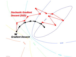
Stochastic Gradient Descent (SGD)

SGD performs parameter update for each instance (data training example and label) one at a time (batch size = 1). SGD implements more frequent updates with high variance. It causes the objective function to vary more intensely, which helps to find more optimal local minima. With every iteration, we need to shuffle the training set (in order to create a pseudo randomness) and pick a training example at random. "Stochastic" signifies that one example, which makes up each batch, gets selected at random.


SGD

The problem with SGD is: since we're using one training instance at a time, the path to the local minimum is going to be noisy, which means the path would be more random.


sgdpaths2_320x240

picture source


An improvement would be a Mini Batch Stochastic Gradient Descent, where we can decide the size of a batch with training examples to perform an update upon.

Mini Batch Gradient Descent:

1 < Batch Size < Size of the entire training set

Mini-batch SGD is good for noise reduction in SGD, nevertheless is still more efficient than the full batch version because it is more effective to compute the loss function on a mini batch SGD than on the entire training data.

Popular batch sizes are: 32, 64, 128 samples.


The Drawback of Gradient Descent

One major problem in Gradient based models and backpropagation is called "vanishing gradient". As we go further and calculate our gradient steps, the value of a gradient will consequently "vanish". That means, the gradient becomes vanishingly small, which blocks the weights from changing its value. Thus, if weights stay unchanged, the neural network stops to learn.


There are more Gradient Descent based optimization strategies. You can have a look at some of them at Google's TensorFlow.

siegel.work

It's AI Against Corona

2019-nCoV There has been a lot of talking about the new corona virus going around the world. Let's clear up some things about it first and then we will see how data science and ai can help us fight 2019-nCoV. ...

Activation Functions

What are activation functions in Neural Networks? First of all let's clear some terminology you need in order to understand the concept of an activation function. ...

Backpropagation

or backward propagation of errorsis another supervised learning optimization algorithm. The main task of the backpropagation algorithm is to find optimal weights in a by implementing optimization technique. ...

CNNs

The Convolutional Neural Network (CNN) architecture is widely used in the field of computer vision. Because we have a massive amount of data in image files, the usage of traditional neural networks wouldn't give much efficiency as the computational time would expl...

Early Stopping

In this article we will introduce you to the concept of Early Stopping and its implementation including code samples. ...

GAN

Generative Adversarial Networks (GANs) are a type of unsupervised neural networks. The network exists since 2014 and was developed by and colleges. ...

Introduction to Statistics

Part III In this third and last part of the series "Introduction to Statistics" we will cover questions as what is probability and what are its types, as well as the three probability axioms on top of which the entire probability theory is constructed. ...

Introduction to Statistics

Part I In the following three parts we will cover basic terminology as well as the core concepts from statistics. In this Part I you are going to learn about measures of central tendency (mean, median and mode). In the Part II you will read about measures of variabili...

Introduction to Statistics

Part II In this part we will continue our talk about descriptive statistics and the measures of variability such as range, standard deviation and variance as well as different types of distributions. Feel free to read the Part I of these series to deepen your knowle...

Logistic Regression

Logit Regression Logit regression is another shortened name derived from logistic unit. Logistic regression is a popular statistical model that generates probabilities for binary classification tasks. It produces discrete values and its span lies in the range of [...

Loss Functions

When training a neural network, we try to optimize the algorithm, so it gives the best possible output. This optimization needs a loss function to compute the error/loss of the model. In this article we will gain a general picture of Squared Error, Mean Sq...

The Magic Behind Tensorflow

Getting started In this article we will delve into the magic behind one of the most popular Deep Learning frameworks - Tensorflow. We will look at the crucial terminology and some core computation principles we need to grasp the real power of Tensorflow. ...

Classification with Naive Bayes

The Bayes' Theorem describes the probability of some event, based on some conditions that might be related to that event. ...

Neural Networks

Neural Networks - Introduction In Neural Networks (NNs) we try to create a program which is able to learn from experience with respect to some task. This program should cons...

PCA

Principal component analysis or PCA is a technique for taking out relevant data points (variables also called components or sometimes features) from a larger data set. From this high dimensional data set, PCA tries extracting low dimensional data points. The idea...

Introduction to reinforcement learning

Part IV: Policy Gradient In the previous articles from this series on Reinforcement Learning (RL) we discussed Model-Based and Model-Free RL. In model-free RL we talked about Value Function Approximation (VFA). In this Part we are going to learn about Policy Based R...

Introduction to Reinforcement Learning

Part I : Model-Based Reinforcement Learning Welcome to the series "Introduction to Reinforcement Learning" which will give you a broad understanding about basic (and not only :) ) techniques in the field of Reinforcement Learning. The article series assumes you have s...

Introduction to Reinforcement Learning

Part II : Model-Free Reinforcement Learning In this Part II we're going to deal with Model-Free approaches in Reinforcement Learning (RL). See what model-free prediction and control mean and get to know some useful algorithms like Monte Carlo (MC) and Temporal Differ...

Recurrent Neural Networks

RNNs A Recurrent Neural Network (RNN) is a type of neural network where an output from the previous step is given as an input to the current step. RNNs are designed to take an input series with no size limits. RNNs remember the past states and are influenced by them...

SVM

Support Vector Machines If you happened to have a classification, a regression or an outlier detection task, you might want to consider using Support Vector Machines (SVMs), a supervised learning model, that builds a line (hyperplane) to separate data into groups....

Singular Value Decomposition

Matrix factorization: Singular Value Decomposition Matrix decomposition is another name for matrix factorization. This method is a nice representation for applied linear algebra in machine learning and similar algorithms. ...

Partial Derivatives and the Jacobian Matrix

A Jacobian Matrix is a special kind of matrix that consists of first order partial derivatives for some vector function. The form of the Jacobian matrix can vary. That means, the number of rows and columns can be equal or not, denoting that in one case it is a squa...

Introduction to Reinforcement Learning

Part III: Value Function Approximation In the previous Part I and Part II of this series we described model-based and model-free reinforcement learning as well as some well known algorithms. In this Part III we are going to talk about Value Function Approximation: w...

Weight Initialization

How does Weight Initialization work? As a general rule, weights and biases are normally initialized with some random numbers. Weights and biases are extremely important model's parameters and play a pivot role in every neural network training. Therefore, one should ...

Word Embeddings

Part 1: Introduction to Word2Vec Word embedding is a popular vocabulary representation model. Such model is able to capture contexts and semantics of a word in a document. So what is it exactly? ...

Word Embeddings

Part 2: Word2Vec (Skip Gram)In the second part of Word Embeddings we will talk about what are the downsides of the Word2Vec model (Skip Gram...

t-SNE

T-Distributed Stochastic Neighbor Embedding If you do data analysis, machine learning or some other data driven research you will prob...
Copyright © 2024 by Richard Siegel at siegel.work Donate Contact & Privacy Policy