Let's sort out everything we've learned so far.

In Part I we learned about model-based RL where we need a model of the environment. The model is often the reward function and the transition probability table with all steps the agent would take. So the environment is defined. But keeping the track of such models might become computationally expensive. We also have to somehow store a potentially infinite amount of states if we account for continuous environment cases. This would explode the time complexity of the model. Thus there is another way ...

... In Part II we tackled model-free RL which has no model of the environment. In such settings the agent would learn from its own experience gathered in the environment. Hence initially the agent has no defined knowledge of the environment. The agent has to figure out by itself what the environment is and what actions are suitable for which states.

Lastly in Part III of this series we handled the topic of Value Function Approximation (VFA) and why we need it. VFA allows us to represent continuous state spaces and to generalize states well.

In this closing Part IV we will look at Policy Based methods in RL. Policy Based RL belongs to a family of model-free methods together with Value Based techniques as well as Actor-Critic methods.

There are two major branches in the picture above: Policy Based methods and Value Based methods. There is also the Actor-Critic methods which is a blend of both Policy and Value based methods.

As a quick recap: a policy π is a probability distribution, which the agent uses to choose actions. We can use a deep neural network to approximate the agent's policy π. The neural network that we chose, will take in observations from the environment and output actions:

The actions are selected according to the Softmax activation function. More on Softmax later in this article. We then create an episode where the agent keeps track of states, actions and rewards in its memory. When an episode ends, the agent goes back through all states, actions and rewards and computes the so called discounted return at each time step (read more on discounted returns in Part II of this series). Now we can use the returns as weights and actions as labels to backpropagate and update the weights of the neural network.

Let's focus on Policy Based methods for a moment. The goal of policy based methods lies in updating the parameters θ such that the expected return (=reward) will be maximized. The advantage of policy based methods is that they use stochastic policies which provides natural exploration. If in Q-Learning (value based) we have to select the optimal epsilon ε in order to choose an action to achieve a certain exploration level, with policy gradient we have automatic exploration.

Example: what if you create an agent which competes another agent in the game of rock-scissors-paper? You want of course that your agent wins. But if the policy of your agent is deterministic, the opponent is able to calculate your next move. Hence you want a policy for your agent that is as random as possible, so that your agent becomes unpredictable for the opponent.

Let's have a look at another example. We have an environment and some deterministic policy π for our agent. Then our agent might have a problem: it will quickly get stuck between two states never reaching the reward.

the agent gets stuck in the two states marked in violet.

We can solve this problem by introducing a stochastic policy. Following this policy, the agent will randomly move east or west and finally reach the reward.

the agent can better explore other states from states marked in blue.

But we still have a problem: the agent cannot distinguish between two states marked in blue in the picture above. Those states are aliased states and they appear there due to the partial observability in the environment.

What do we mean by partial observability? Imagine we have a small robot (the agent) that drives along a corridor in the floor number 1. Let's say the floor number 2 has the same width, height and is as long as the corridor in the floor number 1. If our robot appears to be in the floor number 2, it won't be able to tell the difference between the floor 1 and 2.

This is called partial aliasing. Partial aliasing happens in non Markov environments or in other words, in environments that does not satisfy the Markov property.

As a quick recap, what is this Markov property? If the probability distribution of future states is conditioned only on the present state and not the past, we call it a Markov property. Read more on this topic in Part I of this series.

All right, for now we can conclude that for continuous action spaces we'd better use policy based methods to introduce some randomness (to become "unpredictable"). If we use value based methods for continuous actions spaces, we quickly have the following problem: for each (action,state)-pair we have to store some value in the memory. If we receive a million actions, it becomes computationally expensive to evaluate the action that brings the maximum reward. The action evaluation becomes intractable as we have to calculate the value for each possible action which in turn might go into millions.

So if we have a robot moving in different directions, it is better to find the policy π(state, action) directly by applying policy based methods.

Policy Based Methods: Better Convergence

With policy based methods we achieve a better convergence for the model:

1. we find the policy π
2. then we find the gradient
3. we optimize the policy by moving towards the gradient
4. and finally we update the policy π based on the gradient

Now let's summarize advantages of policy based RL methods. A policy based RL allows:

1. better convergence
2. to be effective in high dimensional spaces
3. learning stochastic policies

Possible disadvantages of policy based RL would be that such model will converge to a local and not global optimum. Moreover, the agent discards previous experience and learns from scratch in each new episode. Also evaluating a policy will lead to high variance and ineffectiveness of the model.

Still, in general it is easier to follow the given policy π than computing the value function.

High Variance with Policy Based Methods

The question we might ask is: why does the variance of policy based methods get high? High variance between episodes happens due to the fact that each time the agent visits some state, the agent can choose different actions, which in turn leads to different future returns (=discounted sum of rewards G).

How do we deal with high variance in policy based methods? We can scale rewards by a baseline. The idea behind the baseline is to subtract from G (=discounted rewards) some baseline-amount b(s) in order to reduce the changes in results.

An example of a simple baseline would be averaging all the rewards we get from an episode and then normalizing the sum of discounted rewards G by using this average: we now can divide by the standard deviation of all rewards from an episode and thus control the variance of rewards.

Why is a stochastic policy better?

A stochastic policy is better:

1. in antagonistic environments or in other words, in cases where an action might be predictable (like in rock-scissors-paper)
2. in partially observable environments where the agent needs to try out different actions, so it won't stuck in two states for ever.
3. in cases of continuous actions spaces.

Softmax Policy

The Softmax Policy is a softmax function that converts output to a probability distribution. That means, the softmax function influences the probability of each possible action.

We normally use softmax in discrete action spaces.

We can try to compute the policy gradient analytically. That means, we assume that the policy π is differentiable in each non zero point. We also know the gradient.

The Gradient

The gradient of a policy π looks as follows:

Likelihood Ratios

The property shown in the equation above is called likelihood ratios.

And this part of the equation:

is called score function .

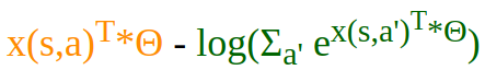
Example : Softmax policy π_Θ parameterized by Θ is defined as follows:

where x(s,a) is a feature vector for state s and action a , T is Time step , Θ is a weight vector and A is a set of all possible actions.

Given that, what is the corresponding score function?

The corresponding score function will look like this:

When derived, this score function has the following form:

Note: the part marked in blue obeys the following property:

Let's take the derivatives of the inner function * the derivatives of the outer function by applying the chain rule:

If we look at the same equation once more, we can see the hidden policy π_θ(a|s) :

Now we can rewrite the equation above as:

The part of the equation marked in orange is the expected value of the feature vector if the agent takes any action. Let's take a quick look at the definition of Expectation :

where X stands for features and P for probability.

So we can write the equation marked in orange as follows:

Gaussian Policy

With continuous action spaces we apply Gaussian policy, so we can sample actions from the Gaussian distribution:

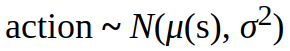
The score function of the Gaussian Policy looks like this:

where a stands for action, μ(s) for mean and σ² for standard deviation.

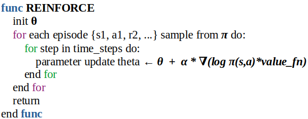
REINFORCE or Monte Carlo Policy Gradient

In the REINFORCE algorithm we have no Q values as a "middle man", instead we find the policy directly:

1. we update our parameters by applying Stochastic Gradient Descent SGD
2. then we sample expectation to get a reward per episode
3. and lastly we update parameters for each step in the episode.

Conclusion

Policy Based Methods in Reinforcement Learning are methods that optimize the policy directly. Instead of working with value functions, these methods work directly with the policy. With policy gradient we answer the question: how can we analyze experience and from this analyzed experience figure out in which direction we should adjust the policy.

In general we adjust the policy by following the gradient as our optimization tool.

Further recommended readings:

Part I : Model-Based Reinforcement Learning

Part II : Model-Free Reinforcement Learning

Part III : Value Function Approximation