As a small recap: In reinforcement learning our main task is to figure out an optimal policy π . An optimal policy π is an "instruction set" for the agent so it knows how to act in order to maximize the total return (=reward) in every state.

There are often situations in Reinforcement Learning (RL) where it is difficult to apply a Markov Decision Process (MDP: read more about MDPs in Part I). For example, we generally have no idea how exactly the environment, where the agent acts, works or computing the transition probability function might be computationally expensive or in some cases even impossible. Shortly speaking, it is not an easy task to find a model of an environment. That is why, we might want to find out how we can go along without using a model. Model-Free Reinforcement Learning comes to the rescue.

The Model-Free RL approach uses no transition probability table and no reward function. Those two are often called "the model" of the environment. If we omit them, we get a "model-free" method.

We can exclude the model and let the agent learn from observed experience straight forward. In other words, instead of finding a model, we use model-free algorithms and allow the agent to learn while it acts without explicit knowledge of the environment - without any model, hence model-free.

Exploration and Exploitation

On a very high level, if the agent has to figure out itself how to behave, we have to give it some freedom (exploration) and some rule-set (exploitation).

We can increase the level of exploration in the agent and then it will try new actions all the time. The positive side is that the agent might potentially discover actions that might be very beneficial for its learning and result. The negative side is that the agent explores so much, it might ignore the actions that are optimal already. The agent keeps trying out all possible new actions that might be worse.

An exploration example would be an ε-greedy (epsilon-greedy) policy which can explore too much if tuned falsely. ε-greedy acts greedily in most cases, but sometimes it randomly chooses one action from all possible actions for exploration. How often the algorithm chooses random actions is defined by the parameter ε epsilon, hence ε-greedy. By doing so the algorithm considers new actions during sampling. For example, take two extremes: with probability ε = 1 the algorithm chooses a random action, hence the agent behaves completely explorative. With probability ε = 0 the algorithm chooses a greedy action all the time. This returns maximum reward for a state the agent is in. Hence ε of 0 means the agent is completely exploitative.

Exploitation, on the other hand, is another extreme: when the exploitation level is high, the agent keeps doing what it was doing all the time and trying out nothing new. By having high exploitation, the agent oversees other actions that might be more beneficial than those the agent chooses again and again. Nevertheless, the positive side is that the agent has a certain trajectory (an episode) and an action-set which was proven to work. But if it tries nothing new, it will never learns whether there are better possibilities or not.

An example here would be a greedy policy. The greedy way of training an agent includes locking an agent on one action that acquire good results in the past. With the greedy policy the agent doesn't explore, instead it only exploits this one action while ignoring other potentially better actions in order to maximize the immediate reward. Hence it exploits too much, which still might be more useful in some applications.

An approach to tackle the exploration vs. exploitation trade-off problem is introduced in the so called decaying ε-greedy policy. A decaying ε-greedy policy decreases the exploration percentage as the training time goes by. In other words, the agent starts off the learning with high exploration and with time after it explored enough it goes to exploitation.

On Policy vs. Off Policy

On policy means that the agent strictly follows the given policy π all the time and can select actions as it wants. The on policy mode gives the agent a certain plan to trail, in consequence the steps are obvious for the agent. Basically, with an on policy learning the agent learns its policy by sampling from the same policy. This sampling from the same policy might become a problem in some use cases because in some applications it is better that the agent observes behavior of another policy (e.g. of another agent) to find an improved policy. An off policy learning might be a solution.

An off policy mode optimizes the target policy by learning from samples which were generated by a different behavior policy (e.g. by a different agent). For example, we have a robot called Jimmy. With an off policy mode, the robot Jimmy will observe another robot called Sam performing some actions. So Jimmy learns how to "behave" from Sam.

Besides, an off policy learning allows the agent to learn the optimal policy by doing more exploration. With an off policy learning the agent can learn about multiple policies while following one policy.

Bootstrapping

In Part I of this series we talked about Dynamic Programming (DP) methods. DP methods update the current estimates of states based on estimates of successor states. Meaning DP methods update estimates based on other future estimates. This concept is called bootstrapping.

Not only model-based reinforcement learning methods utilize bootstrapping. Temporal Difference, TD-Learning, is model-free and uses bootstrapping as well.

On the other hand, Monte Carlo, MC-Learning, is also model-free but uses no bootstrapping (more on TD/MC-Learning methods down below).

Those general rules are not set in stone. Depending on the application and experimentation these properties can be blended in interesting combinations.

We will look at more examples of how bootstrapping works in the next Part III of this series.

For more information consider Reinforcement Learning: An Introduction, Richard S. Sutton and Andrew G. Barto from page 89.

Let's go through some important model-free techniques.

Given some policy π, we want to predict future rewards (sometimes called Utility) given an action set S. But because we have no environmental model (no transition probability distribution and no reward function) we cannot compute the expectation E directly. That means, we have to sample from the environment and iteratively estimate the value function. There are two main RL model-free techniques to do that: Monte-Carlo (MC) Learning and Temporal Difference (TD) Learning.

Monte Carlo (MC)

Generally speaking, Monte Carlo (MC) methods are a set of model-free algorithms (=the agent does not know MDP state transitions) that rely on repeated random sampling. A MC algorithm applies randomness in order to solve problems that could be deterministic - it uses repeated random sampling as basis for obtaining statistical results.

Monte Carlo methods are named after the notoriously known gambling city in Monaco. Because random outcomes are prior to Monte Carlo techniques there is a clear correspondence to games like dice, roulette, slot machines, etc...

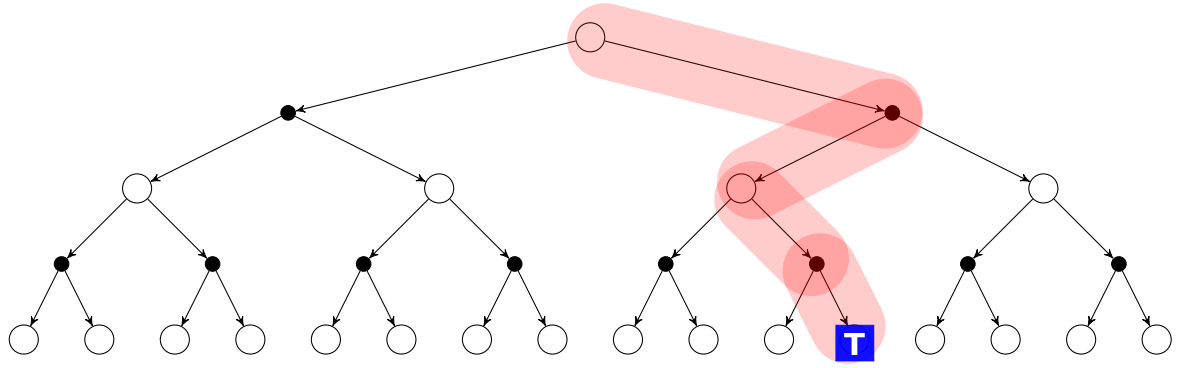
In the world of Reinforcement Learning, the MC Learning samples complete episodes and updates the found mean of all states afterwards. MC can learn on complete episodes only, hence it must wait till the end of an episode before the return is known. Moreover, all episodes must terminate at some point and cannot go on forever as e.g. in some games that you can potentially play continuously. There is also no estimate about the future - bootstrapping is not used.

You can see the MC backup strategy on the picture below:

MC update equation:

V(S_t) ← V(S_t) + α(G_t - V(S_t))

where G_t is the MC target:

A backup strategy shows how an algorithm updates the value of a state using values of future states.

We previously said that MC learns the state value V_π(s) function under a policy π by analyzing the average return from all sampled episodes (the value is the average return).

To make it more clear, MC learning can be compared with an yearly exam - the result of the exam is the return acquired by the student (=agent), so the student completes an episode at the end of the year.

Imagine we want to know students' performance during the year which can be seen as an episode. We can sample results of some students and then calculate the mean result to find the mean student studying performance.

Now let's look at two major steps in MC-Learning:

1. Monte Carlo Prediction (=MC policy evaluation):

We estimate V_π(s) - the value of a state under some policy π - given episode set that we gathered following the policy π . A visit to the state s is an occurrence of this state s in one episode. The agent is allowed to visit the state s multiple times during one episode. The first time the agent visits a state s is called the first-visit MC. The first-visit MC calculates V_π(s) as the return average according to the first visit to the state s.

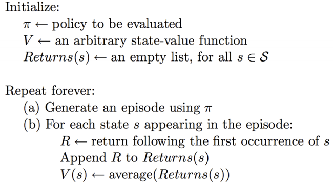
First-Visit Monte Carlo Policy Evaluation

Note: there is also the Every-Visit MC method which averages the returns according to all visits to s.

2. Monte Carlo Control (=MC policy improvement)

In this step we are ready to optimize the policy. The question is: how can we utilize Monte Carlo estimation control, so that we can approximate an optimal policy.

Conclusion: MC Learning can only be applied to episodic problems and the episodes must terminate in order to be complete.

Temporal Difference (TD) Learning

TD learning combines the best of both Monte Carlo (MC) and Dynamic Programming (DP).

1. TD methods learn directly from experience without a model of the environment, exactly like Monte Carlo techniques do.

2. TD methods also update estimates based on other learned estimates, they also do not wait for the final outcome, hence TD methods bootstrap, exactly like Dynamic Programming does.

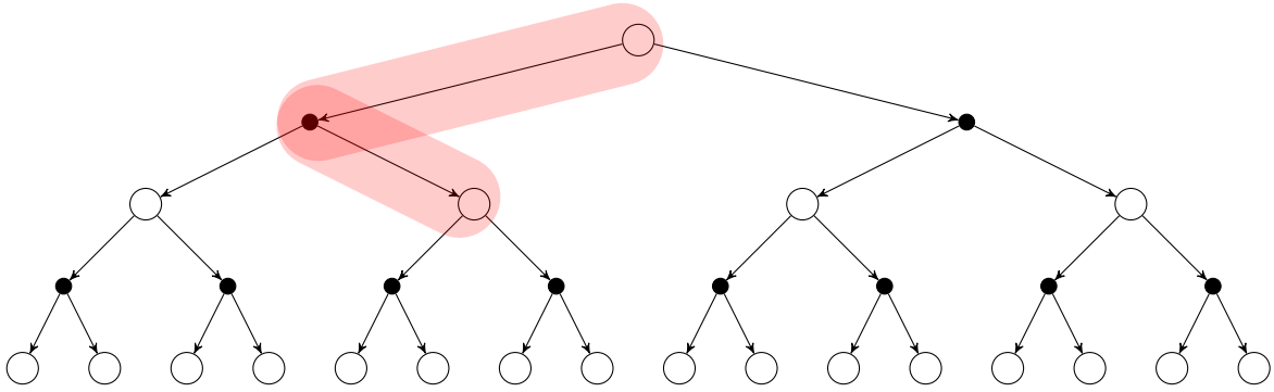
TD Learning samples one step, hence it learns from incomplete episodes and updates the estimate by the direct reward and the current estimate of the next step.

You can see the TD backup strategy on the picture below:

TD update equation:

V(S_t) ← V(S_t) + α(R_t+1 + γV(S_t+1) - V(S_t))

where R_t+1 + γV(S_t+1) is the TD target:

Summary: MC vs. TD Learning

TD and MC: Bias and Variance

To understand what the bias-variance tradeoff in reinforcement learning means, let's first go through some basic ideas underneath bias and variance.

Bias

In our context bias means the inability of a machine learning model to express the true relationship between the data points.

Variance

We talk about high variance if the model fits the training data set too well. The model fits the data so well that it fails to generalize to the new unseen data (=test set). The cause of high variance often happens because the model learns the noise in the data as patterns.

To estimate V_π(s) value function, we update V_π(s) with the following equation:

V_π (s_t) ← V(s_t) + α(Target - V_π (s_t))

With each update of V_π(s) we take a step towards the target. The target can be the Monte Carlo Target or Temporal Difference Target.

The Monte Carlo Target = the return G_t .

This equation shows the discounted sum of rewards from each state s until the end of an episode.

Because the MC target:

Temporal Difference Target : because TD does not wait until the end of an episode (like MC does), the Target = immediate rewards plus estimate of the future rewards:

R_t+1 + γV(S_t+1)

Notice in the equation above we apply bootstrapping: we use an estimate to update the current estimate value.

Bias-Variance Tradeoff with TD and MC

When we talk about bias and variance of MC and TD Learning, we talk about bias and variance of their target values.

In most circumstances, our agent cannot exactly predict the results of its actions, hence there is no precise calculation of the state or action values. That is why the agent estimates these values iteratively. At this estimation step the notion of bias and variance is significant.

With Monte-Carlo learning the agent uses complete episodes (=complete trajectories). For every step in an episode we calculate a state value. But our main problem with MC is that the policy and the environment are both stochastic (=random). This means, some noise is introduced. The stochastic nature of both the environment and the policy creates variance in the rewards acquired in one episode.

As an example, imagine that we have a small robot. The goal of this robot is to reach the end of a corridor. If it completes the task, it receives a reward. Now imagine that the policy of our robot is stochastic. We could have cases in which the robot can accomplish the task successfully. But in other cases it might fail to do so. In the end, when we compare the overall results, we will see that we have very different value estimates because of very different possible outcomes. We can potentially reduce variance by utilizing a large number of episodes. Then we hope that the variance introduced in any one specific episode will be lessen and will provide an estimate of the true environment rewards.

With Temporal Difference learning the reward is equal to the immediate reward plus a learned estimate of the value at the next step (=bootstrapping). TD counts on a value estimate that stays stable as time proceeds. So, TD is less stochastic.

The other problem with TD is that because TD uses value estimation, the reward value becomes biased. It happens because the estimate stays an estimate (=approximation) and hence can never be 100% accurate.

Let's come back to the corridor-robot example. Let's say, we have a value estimate of the end of the corridor (corridor = environment). The estimate can say that acting in this one corridor brings less reward, which may be false. It occurs because the estimate can not always distinguish between this one particular corridor and other similar corridors which might be less rewarding to act in.

Balancing Bias and Variance

How can we deal with high bias and variance causes? There are many techniques to diminish the negative effect of high bias or/and high variance in the reward. You can read about Asynchronous Advantage Actor-Critic, Asynchronous Methods for Deep RL and Proximal Policy Optimization.

MC and TD Learning bias-variance: Summary

With MC (target G_t) we have no bias but high variance and with TD (target R_t+1 + γV(S_t+1)) we can experience high bias and we have low variance.

Back to TD-Learning

In TD-Learning there are two major algorithms for model free RL, namely: SARSA and Q-Learning.

SARSA

SARSA is an on-policy TD control (=policy improvement) RL algorithm that estimates the value of the policy being followed. It has its name because it uses State-Action-Reward-State-Action experiences to update its Q-values, which are computed by the state-action value function Q. You can learn more about the value function in RL in Part I of this series, but as a quick recap in RL we want the agent to find the state value function V_π(s) or the action value function Q(s,a). These both value functions indicate how much reward a state s and an action a will bring.

What is the basic idea behind SARSA?

For every step the SARSA algorithm performs:

1. policy evaluation:

policy update + evaluation based on ε-greedy configuration.

Q-Learning

Q-Learning is an off-policy TD control (=policy improvement) RL algorithm. The Q-learning function learns from actions that are not part of the current policy (e.g. it chooses actions randomly), so there is no need for a policy, hence Q-Learning is an off policy method.

What is the basic idea behind Q-Learning?

This type of TD-Learning algorithms wants to find the best action the agent can choose given the current state the agent is in.

Let's do a quick recap and sort out the RL methods learned so far:

To learn more, see Part I

Now let's compare TD-Learning algorithms: SARSA vs. Q-Learning

SARSA

1. on policy learning

2. looks for the next policy value

3. in general: "more conservative" - tries to avoid dangerous not known paths with potential negative (but also potential positive) reward

Q-Learning

1. off-policy learning

2. looks for the next maximum policy value

3. in general: more explorative - tires out new ways to find the optimal path

RL Algorithm Structure

Basically the structure of most RL algorithms looks the following way:

1. model free prediction: this is our policy evaluation step - here we compute the state value function V_π .

Example algorithms:

Monte Carlo Learning : the agent learns from complete episodes

Temporal Difference Learning : the agent learns based on bootstrapping

2. model free control : this is our policy improvement step - here we approximate the optimal policy.

What we do:

1. tweak on exploration/exploitation
2. choose either an on-policy learning (SARSA) or ...
3. ... an off-policy learning (Q-Learning)

Further recommended readings:

Part I : Model-Based Reinforcement Learning

Part III : Value Function Approximation

Asynchronous Advantage Actor-Critic