Matrix Factorization: Definition

A matrix factorization is a mathematical method that "breaks down" (decomposes) a matrix into its separate integral components.

It is a process that can make more complex matrix operations easier by "splitting up" an initial matrix into some consistent pieces, so that those operations can be performed on the decomposed matrix (those "pieces") and not on the original one, more complex, matrix.

Factorization:

Consider the factoring of a natural number e.g. 20 into 2 * 10. That means, that 20 is a composite number and we can decompose (factorize) it into some pieces (2 and 10), which multiplied still represent the initial number 20. So you can think of a matrix factorization as "dividing" a big composite matrix into some smaller ones, which are less complex intrinsically.

There exist different methods to factorize (decompose) a matrix. For now, we will focus on one of them called SVD or Singular Value Decomposition.

Singular Value Decomposition (SVD): Introduction

SVD stores only important information in order to have a dense vector with a low number of dimensions. That means, SVD is one of many dimensionality reduction techniques.

Dimensionality Reduction

We need dimensionality reduction to overcome the so called Curse of Dimensionality. If the number of dimensions in data increases, the distances between the data points increase as well, which leads to a higher sparsity in the data set. Even the closest neighboring points are too far away from each other. That means, with more dimensions, we need more data. More data means, computation time increases as well as more storage capacities are required. The problem becomes computationally expensive.

One further problem with a large number of dimensions is, it is difficult (nearly impossible) to visualize let's say, 1000 dimensions in a way that a human being is able to understand it. Humans can only see up to 3 dimensions. Fortunately, with SVD we can present our data in lower dimensions and visualize it much easier.

Some Dimensionality Reduction Techniques include: Random Forest, Principal Component Analysis (PCA), t-Distributed Stochastic Neighbor Embedding (t-SNE), Singular Value Decomposition (SVD) and many more.

Visualization of SVD:

watch the visualization here.

Singular Value Decomposition (SVD): Definition

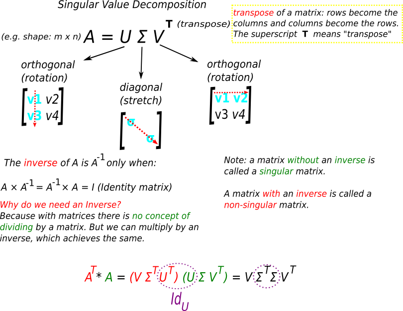
For a start, we have a matrix A which we want to decompose. A is our initial data matrix. When we decompose the A matrix, we get the following three matrices: U, Σ and V^T. With SVD we decompose the matrix A into a product of three matrices. (Note: V^T means the transpose of a matrix. A transposed matrix is a new matrix, where the rows are the columns of the original matrix).

decomposing the A matrix :

the transpose of a matrix :

Singular Value Decomposition (SVD): Geometric way of thinking

UΣV^T as a result of the origin data matrix A is possible due to linear algebra and linear transformation. U, Σ and V^T are a representation of some "movement" (transformation) in a linear space. This "movement" is mostly done by addition and scalar multiplication and can be: scaling, rotation or reflection.

Let's transform our three matrices (UΣV^T) into its original one A

V^T : rotation and reflection

We multiply some matrix B by V^T :

BV^T and we get a new matrix.

Σ : scaling

Σ * (V^TB)

because Σ has values (singular values) on the diagonal, it only scales the matrix. Scaling means an operation which stretches or squishes the matrix (or a vector).

U : rotation and reflection

U * (Σ * ( V^T*B) )

Finally, we rotate and reflect the Σ*(V^T*B) matrix with the help of U and we get our original matrix A

if you'd like to know more about Linear Algebra or refresh you knowledge, you can watch this playlist from the YouTube channel called 3Blue1Brown

Properties of U, Σ and V^T

The initial A matrix is still close to one of the three newly created matrices (U, Σ or V^T). That means, when we find a low rank matrix, it can serve as a good approximation of the initial decomposed data matrix (in this case A).

Clarifying U, Σ and V^T

U, Σ and V^T are also unique matrices, meaning one cannot be a replica of another.

U, V are orthogonal, which means, if we take two columns of U (or V) and multiply them together, we get 0. And they are also column orthonormal. Orthonormal means, the columns' length equals 1 (unit length\unit vector). Unit vector is sometimes called "direction vector" because it describes only the direction of a vector, not its magnitude.

Σ is a diagonal matrix: the entries are on the diagonal line and are sorted in decreasing order. The entries are also only positive numbers.

What do the numbers in U, Σ and V^T matrices actually represent in the real-world data?

As an example, we can take our A matrix and say that it is of the form [m x n]. Now we can specify that, m (rows) represents documents in a corpus and n (columns) represents words from those documents. That is one of possibilities, what the matrix A could stand for in the real-world data representation.

what about the rest?

If we want to bring in our data, which is a bunch of words from some documents (the A matrix) and we categorize the words, we can say that:

1. U represents the relation between a word a category (could be e.g. word embeddings)
2. Σ represents the strength of the categories
3. V represents the relation between a document and a category

With the help of SVD, we can also build a recommender system to suggest movies based on users' ratings. Our matrices would be the following representations:

1. U represents the relation between a user and a concept (Note: a concept here means a movie genre: comedy, drama, thriller...) (could be e.g. word embeddings)
2. Σ represents the same as before strength of the concepts
3. V represents the relation between a movie and a concept

Dimensionality Reduction with SVD

The following procedure decreases the complexity of the data:

set the smallest singular values in Σ to 0. That means, take the column from U, which corresponds to the column in Σ with the smallest singular value and set this column from U to 0. Take the corresponding row of V^T and set it to 0.

SVD and Eigenvalue Decomposition

Singular value decomposition can decompose a matrix of any dimension. SVD can be applied to any m x n or m x m matrix. On the other hand, eigenvalue decomposition can be applied only to matrices with a clear diagonal line, that means, the matrix must be square (m x m).

Column vectors in one matrix from Eigenvalue Decomposition are not necessarily orthogonal, which means it doesn't always represent rotations/reflections. U and V in SVD are always orthogonal and always represent rotations and reflections.

The singular values in Σ are all real and non-negative numbers. The eigenvalues in Eigenvalue Decomposition can be complex and even have imaginary numbers.

Summing everything up ...

Conclusion

SVD is one of the most widely used techniques for dimensionality reduction, recommender systems, object recognition, risk modeling and many more other models. SVD combines the main linear algebra concepts, namely: matrix transformations, projections, change of basis, symmetric matrices, orthogonality and factorization.

The problem with SVD is that for an n x m matrix the time complexity will be quadratic: O(mn²)

Further recommended readings/courses:

Principal Component Analysis (PCA)

Singular Value Decomposition (SVD)

MIT Open Courses "Linear Algebra"