Backpropagation
The context of Backpropagation
What is the role of the Backpropagation algorithm and when do we need it? We use Backpropagation in the context of Neural Networks in he following algorithmic procedure:
- Forward Propagation
- Computing the Loss / Cost Function
- Applying Backpropagation
And still why do we need backpropagation specifically? Why not just use a Feed Forward approach? We will first need some background knowledge to answer this question.
Feed Forward
Feed Forward Neural Network is the basic model of an artificial neural network. It is often used for regression and classification tasks. There is no looping in the feed forward model, that is why a feed forward neural network is called so. There is only a forward flow of the information. The model takes in some input on the input layer level. Then it "feeds" this input to the hidden layers (there may be many of them). Subsequently, the calculation is forwarded to the output layer. All in all, data flows in only one direction from input through hidden layers to the output.
The data flow happens because each layer in a neural network is connected with each other by weights. Each neuron in a feed forward neural network receives a set of inputs, performs a dot product, and then applies an activation function to it. Then we just repeat that process to output a prediction.
After that we compare the prediction with the desired output. It can be seen then, that our prediction is incorrect, which means that the weight values are not optimally calculated. Consequently, we want to find the best weight values in a way that, given any input, the correct output will be calculated with the help of the optimally calculated weights. Our main goal is to minimize the found error and we can do it with the help of the algorithm called gradient descent. More on gradient descent here.
We use gradient descent to increase the accuracy of the model's prediction. Backpropagation has its name because we propagate the derivatives back through the network and at the same time we update the weights accordingly.
Small Recap on Calculus
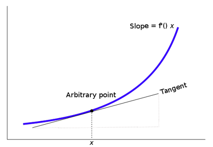
a derivative (d) is a slope of some tangent line which is on a curve at a specific point. A derivative measures the function's instantaneous rate of change:
a partial derivative is a function with several variables:

A partial derivative of a function with several variables is its derivative with respect to one of those variables with the others kept constant.
Gradient
Backpropagation is an algorithm for computing partial derivatives (the gradient) of the loss function.
Gradient (∇) is a vector of partial derivatives. In other words, we organize partial derivatives in this special vector called gradient.
Example of a gradient :
-∇C (w, b, …) = [0.17, 0.20, 0.03, 0.52, 1.72, ...]
Each value in the vector represents sensitivity of the connections (weights).
The concept of differentiation (derivative / partial derivative) is widely used in other mathematical idea used in Backpropagation, called the Chain Rule. Backpropagation is basically an algorithm that computes the chain rule.
The Chain Rule
A neural network is in its essence a big composite function. If we come back to the feed forward model, we can see that each layer of a single neural network can be represented as a function.
We can also compute derivatives of composite functions. A composite function is a function, which consists of another functions. That means, we may have a complex function that is composed of multiple nested functions.
The chain rule is used to compute partial derivatives that are stored in the gradient of the error function with respect to each weight.

The Chain Rule: algorithmic procedure
- take the derivative of a "sub-function"
- take the derivative of the entire function
Example:

Back to Backpropagation
The purpose of backpropagation is to figure out the partial derivatives of the error function with respect to the weights in order to use those in gradient descent.
That means, we backpropagate to update weights with the help of gradient descent.
Backpropagation utilizes the Chain Rule to increase efficiency. Firstly, we go forward through the whole network once. Secondly, we move through the network backwards once. By passing the network forwards and backwards we can compute all the partial derivatives we need to calculate the error. The nice part is: computationally, backpropagation takes approximately the same time as if we complete two forward passes through the network.
After we determined the error for the final output layer, we calculate the error again but this time not for each separate neuron in the hidden layers. We can accomplish this by moving backwards layer by layer in the neural network.
This error for a neuron in the hidden layers looks like this:

We can apply those errors to compute the weights variation:

This operation is repeated for all the inputs and deltas (Δ) are getting gathered and stored:

Finally, when we land at the end of one learning iteration (weights update), the actual (old) weights are changed accordingly to the newly accumulated weights (the change in weights, delta Δ) for all training samples:

Backpropagation: The Algorithmic Thinking
- apply feed forward (derivatives of the activation function are stored in each neuron)
- backpropagate to the output (accumulate all the multiplicative terms, define the backpropagated error)
- backpropagate to the hidden layer (compute the backpropagated error)
- update weights (the weights are updated in the negative direction of the gradient)
An important note is : make the weights adjustments only after the backpropagated error computation. The computation of the backpropagated error must occur for all neurons in the neural network. If you adjust weights before the backpropagated error was computed, the weights adjustment gets twisted with the backpropagation of the error. As a result the calculated adjustments do not correlate with the direction of the negative gradient.
Backpropagation Through Time
You will sometimes hear about "backpropagation through time" or BPTT for short. It is broadly speaking the same as the "normal" backpropagation only with some additional property.
In order to calculate the gradient at the current time step, BPTT will need all the previous gradient calculations. For example, we want to calculate the gradient at the time step 4, so t=4. To do that we need to compute all the gradients from the time steps t=1, t=2, t=3 and sum them up.
As we can see from the example above, to use BPTT is computationally expensive. For example, if we have 10.000 time steps on total, we have to calculate 10.000 derivatives for a single weight update, which might lead to another problem: vanishing/exploding gradients.
Both BPTT and backpropagation apply the chain rule to calculate gradients of some loss function. Backpropagation is used when computing gradients in a multi-layer network. On the other hand, BPTT is applied to the sequential data (time series). BPTT is also widely used in models like Recurrent Neural Networks (RNNs).
Conclusion
To sum it up, the gradient computation proceeds backwards through the entire model. Firstly, the gradient of weights in the last layer is computed. Lastly, the gradient of weights in the first layer is computed. Partial calculations of the gradient in one layer are reused in the calculation of the gradient in the previous layer. Such backwards error flow enables a highly efficient gradient computation at each layer. On the other hand, calculating the gradient of each layer separately has been proven to be less efficient.
To conclude, the main advantage of the backpropagation algorithm in comparison to the feed forward model is that with backpropagation we can calculate all the partial derivatives at the same time utilizing just one forward and one backward pass through the neural network.